Wellcome back!
In this article we will talk about Reinforcement Learning and, in particular, we will discuss about one of the algorithms used in this specific machine learning area, the Q-Learing algorithm.
But first:
What is Reinforcement Learning???
The Reinforcement Learning is a machine learning paradigm and it is about taking a particular action in order to get the highest reward possible in a particular situation.
The concept is not that hard to understand, but to make it easier take as an example a horse and his jockey. Here when the horse moves slowly the jockey will whipe his back.
Otherwise, if the horse starts to accelerate the jockey will give him a sugar lump. So, as soon as the horse understands that by accelerating he will receive a reward he will probably do that more often.
Unfortunatly, in RL we do not have a horse, a jockey or a hippodrome, but we have an software agent (horse) and an environment (hippodrome, jockey) where this agent is located.
Moving on, for a given environment we will have “states” and “actions”. The states are simply observations and informations that we extract from the environment (the velocity and the position of the horse in a particular moment), the actions instead are the possible choices that the agent can make based on the observation (make the horse run or stop).
But…
How do we actually apply RL???
One of the few ways to do RL is using Q-Learning
Q-Learning is a simple model-free algorithm that allows our agent to learn how to succeed within a given environment.
We are going to be working with OpenAI’s gym, specifically with the “CartPole-v1” environment where our objective is to keep a pole straight as long as possible by moving a cart.
To initialize our environment we first MAKE IT (gym.make(“CartPole-v1”)), then we RESET IT (env.reset()) and finally we enter a loop where every iteration we take an ACTION (env.step(ACTION)).
Now let’s explore our environment.
Gym gives us the possibility to query the environment and obtain some really usefull informations.
First we might want to know how many actions are allowed:
import gym

env = gym.make("CartPole-v1")
print(env.action_space.n)
In this environment we can choose between 2 actions: “0” push cart to the left, “1” push cart to the right. This means that whenever we take a STEP we can pass a 0 or a 1, and each time we do so our environment will return us a new state/observation, the reward we obtained, a boolean value telling us whether or not we can keep doing steps and other informations that in our case are irrelavant. So let’s see how our environment works.
import gym
import matplotlib.pyplot as plt
from matplotlib import animation

env = gym.make("CartPole-v1")
env.reset()

done = False
while not done:
    action = 0
    env.step(action)
    env.render()

env.close()
 Here we can see that by just going left or right there is no chance we can achieve our objective, we need to find a way to move the cart left and right so that our pole does not fall. To do that, we could write a function or invent some kind of algorithm, or we can just use Q-Learning!!
Anyways, how will Q-Learning do that?
Once we have discovered the action space we need the observation space. We can get this information when we reset the environment (in this case we get the initial state) and from each step. By printing our observations we would get something like this:
[-0.00403924 -0.3947141   0.04066257  0.6336079 ]
[-0.01193352 -0.59037899  0.05333473  0.93881412]
[-0.0237411  -0.78617784  0.07211101  1.24776774]
This looks confusing but these values are nothing else then: cart position, cart velocity, pole angle, pole angular velocity. The way Q-Learning works is there is a Q (Quality) value per action possible per observation/state. These combinations create a table having for columns the possible actions, for rows the possible observations and in the intersection we have the Q-value telling us how good is to take that action in that specific situation. In order to figure out all the possible states we need to study our environment by either query the environment or explore the environment for a while and figure it out. Luckily, gym gives us the opportunity to get the highest and lowest value of all the attributes that compose the observation space.
low = env.observation_space.low
high = env.observation_space.high
Observation space low: [-4.8000002e+00 -3.4028235e+38 -4.1887903e-01 -3.4028235e+38]
Observation space high: [4.8000002e+00 3.4028235e+38 4.1887903e-01 3.4028235e+38]
Now from these informations we can notice 2 problems:
1-the velocity are continuous, so they do not have a upper bound or a lower bound.
2-the values have 8 decimal places, so having a table with one row per combination would be too high memory consuming, and useless.
So, first thing first we must bring the velocities from continuous values to discrete values and to do that I simply hardcoded the new bounds as -20 and +20, and I choose those values by testing the environment few times (they are not obtimal but they will do the job).
#limit low and high (they will never reach such values)
low[1] = -20.00
high[1] = 20.00
low[3] = -20.00
high[3] = 20.00
Observation space low: [ -4.8        -20.          -0.41887903 -20.        ]
Observation space high: [ 4.8        20.          0.41887903 20.        ]
Coming to the second problem, we want to group the ranges into something more manageable. We will use the “bucketization” by creating some buckets for each range. The number of buckets is a hyperparameter that we might decide to tweak later, but in our case the poles information are way more important than the cart information, so we need more values for the pole’s attributes (that is why in this example we have 50 buckets for pole velocity and position and only 1 for cart position and velocity).
n_buckets = [1, 1, 50, 50]

def get_win_size(os_low, os_high, buckets):
    win_size = (abs(os_low) + abs(os_high)) / buckets
    return np.array(win_size)

np_win_size = get_win_size(low, high, n_buckets)
Win_size: [9.60000038e+00 4.00000000e+01 1.67551613e-02 8.00000000e-01]
The win_size is basically how much we increment the range by for each buckets.
Now we can build the Q-table.
q_table = np.random.uniform(low = 0, high = 1, size = n_buckets + [env.action_space.n])
This is a 1x1x50x50x2 shape and it has random initialize Q-values.
This table is the main component of Q-learning and we will consult with it to determine our moves. The “x2” is our actions and each of those have the Q-value associated with them, but which action we are going to choose? It depends, because we actually have two fases: an “exploitation” fase (or greedy fase) and an “exploration” fase. When we are exploiting the environment we will choose to go with the action that has the highest Q-value in that specific state. At the beginning instead we might want to explore the environment and just go for a random action. This exploration (random actions) is how our “model” will learn better moves over time.
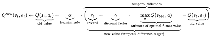
Now we just need to update the Q-table in order to make the learning process possible and we will do so by implementing this easy formula, that can be found here.
 And here the same thing, but coded:
new_q = (1-LEARNING_RATE) * current_q + LEARNING_RATE * (reward + DISCOUNT * max_future_q)
Way less scarry…
The only things that we might not know are: DISCOUNT and max_future_q.
DISCOUNT: a value measuring how much we care about the future reward rather than the immediate reward. It is between 0 and 1 and it is usually very close to 1 because we want our “model” to learn a sequence of actions that leads to a positive outcome, so we put greater importance to the long terms gains rather than short term ones.
max_future_q: it is grabbed after we have performed our action, and then we update our previous values based partially on the next step’s best Q-value. Thanks to this operation the good rewards will get slowly back-propagated leading each episode to possibile higher rewards.
We also need a function that will convert our observations into discrete observations.
def discretizer(obs, win_size):
    discrete_obs = obs / win_size
    return tuple(discrete_obs.astype(int))
We are now ready and have all the knowledge to step through the environment.
First we set our constants (upper case) and variables (lower case)
#Q_learning settings
EPISODES = 70_000
LEARNING_RATE = 0.1
DISCOUNT = 0.95

#Exploration settings (Const)
MINIMUM_EPS = 0.0
START_DECAYING_EPISODE = 10_000

#Exploration settings (Var)
epsilon = 1
reward_threshold = 0
episode_reward = 0
high_reward = 0
prev_reward = 0
epsilon_decay_value = 0.9995
Now we enter the training loop of 70’000 episodes (the number of episodes can be changed), we grab the initial observation from the reset() function and until we are not done (so as long as the pole is strainght or we do not move more than a certain value from the center) we take a step. For each step the action that we will take is based on epsilon. This value will allow us to go from “exploration”, at the beginning, to “exploitation”.
for episode in range(EPISODES + 1):
    done = False
    discrete_obs = discretizer(env.reset(), np_win_size)
    episode_reward = 0

    while not done:
        if np.random.rand() > epsilon:
            action = np.argmax(q_table[discrete_obs])
        else:
            action = np.random.randint(0, env.action_space.n)

        new_obs, reward, done, _ = env.step(action)
        new_discrete_obs = discretizer(new_obs, np_win_size)
        episode_reward += reward
… and if we still good we update our Q-table…
        if not done:
            max_future_q = np.max(q_table[new_discrete_obs])

            current_q = q_table[discrete_obs + (action,)]

            new_q = (1-LEARNING_RATE) * current_q + LEARNING_RATE * (reward + DISCOUNT * max_future_q)

            q_table[discrete_obs + (action,)] = new_q

        discrete_obs = new_discrete_obs
… and when we are done, we have received a higher episode_reward than the previous and we have reached a certain episode (this value can also be changed), we decay our epsilon.
    if epsilon > 0.05:
        if episode_reward >= prev_reward and episode > START_DECAYING_EPISODE:
            epsilon = math.pow(epsilon_decay_value, episode - START_DECAYING_EPISODE)
To check how our agent is doing we print the average, the min and max rewards every 500 episodes and the number of episode that got a reward of 200 or higher.
....
....
10500
EP: 10500 avg: 26.158 min: 8.0 max: 100.0 Objective reached: 0
11000
EP: 11000 avg: 41.628 min: 10.0 max: 352.0 Objective reached: 5
11500
EP: 11500 avg: 67.814 min: 9.0 max: 362.0 Objective reached: 21
12000
EP: 12000 avg: 122.906 min: 10.0 max: 500.0 Objective reached: 98
12500
EP: 12500 avg: 178.376 min: 13.0 max: 500.0 Objective reached: 206
13000
EP: 13000 avg: 212.05 min: 12.0 max: 500.0 Objective reached: 271
13500
EP: 13500 avg: 248.234 min: 12.0 max: 500.0 Objective reached: 376
14000
EP: 14000 avg: 259.318 min: 22.0 max: 500.0 Objective reached: 409
14500
EP: 14500 avg: 258.786 min: 16.0 max: 500.0 Objective reached: 424
15000
EP: 15000 avg: 263.164 min: 24.0 max: 500.0 Objective reached: 439
15500
EP: 15500 avg: 271.57 min: 30.0 max: 500.0 Objective reached: 485
....
....
The graph relative to this particular setting:
epsilon: 1
epsilon_decay_value: 0.9995
Analysis
epsilon: 1
epsilon_decay_value: 0.995
epsilon: 1
epsilon_decay_value: 0.99995
epsilon: 0
epsilon_decay_value: 0.995
From these 3 graphs we can clearly see the importance of epsilon and its decay value. Whithout it we would not have the “exploration” fase and this would not allow our “model” to understand the environment. From this, we can observe the importance of exploration in Q-Learning.